How autonomous vehicle simulation works
Demystifying the virtual test drives that accelerate AV development
When autonomous vehicle developers justify the safety of their driverless vehicle deployments, they lean heavily on their testing in simulation. Common talking points take the form of “we made our car drive X billion miles in simulation.” From these vague statements, it’s challenging to determine what a simulator is, or how it works.

There’s more to simulation than endless driving in a virtual environment.
For example, Waymo’s technology overview page says (emphasis mine):
We’ve driven more than 20 billion miles in simulation to help identify the most challenging situations our vehicles will encounter on public roads. We can either replay and tweak real-world miles or build completely new virtual scenarios, for our autonomous driving software to practice again and again.
Cruise’s safety page contains similar language:1
Before setting out on public roads, Cruise vehicles complete more than 250,000 simulations and closed course testing during everyday and extreme conditions.
The main impression one gets from these overviews is that (1) simulation can test many driving scenarios, and (2) everyone will be super impressed if you use it a lot.
Going one layer deeper to the few blog posts and talks full of slick GIFs, you might reach the conclusion that simulation is like a video game for the autonomous vehicle in the vein of Grand Theft Auto (GTA): a fully generated 3D environment complete with textures, lighting, and non-player characters (NPCs). Much like human players of GTA, the autonomous vehicle would be able to drive however it likes, freed from real-world consequences.
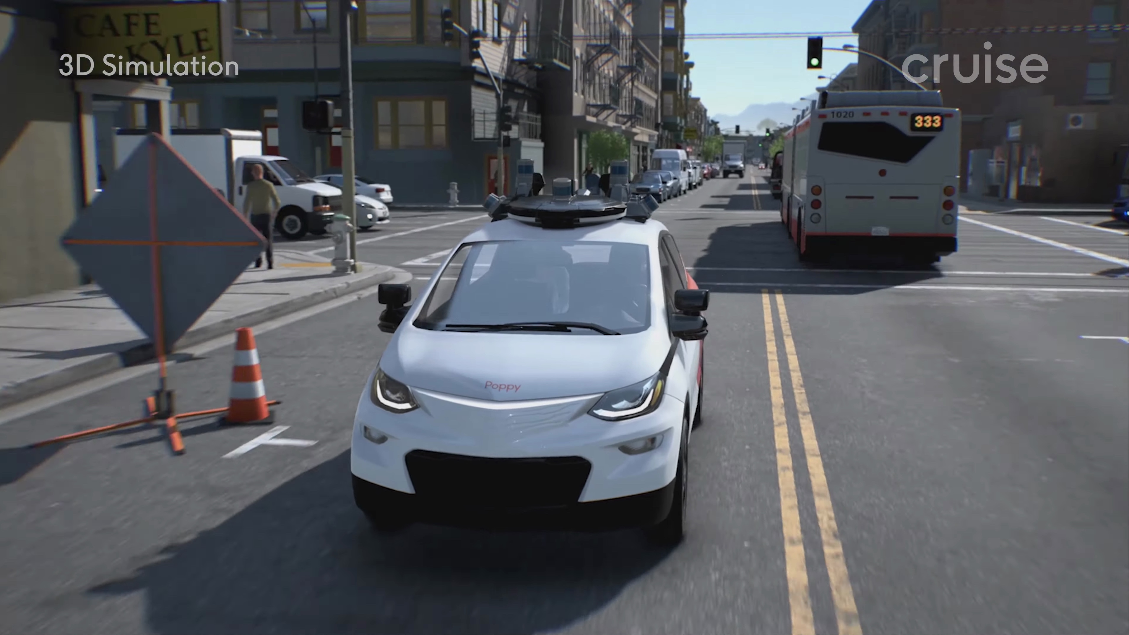
Source: Cruise.
While this type of fully synthetic simulation exists in the world of autonomous driving, it’s actually the least commonly used type of simulation.2
Instead, just as a software developer leans on many kinds of testing before releasing an application, an AV developer runs many types of simulation before deploying an autonomous vehicle. Each type of simulation is best suited for a particular use case, with trade-offs between realism, coverage, technical complexity, and cost to operate.
In this post, we’ll walk through the system design of a simulator at a hypothetical AV company, starting from first principles.
We may never know the details of the actual simulator architecture used by any particular AV developer. However, by exploring the design trade-offs from first principles, I hope to shed some light on how this key system works.
Contents
Our imaginary self-driving car
Let’s begin by defining our hypothetical autonomous driving software, which will help us illustrate how simulation fits into the development process.
Imagine it’s 2015, the peak of self-driving hype, and our team has raised a vast sum of money to develop an autonomous vehicle. Like a human driver, our software drives by continuously performing a few basic tasks:
- It makes observations about the road and other road users.
- It reasons about what others might do and plans how it should drive.
- Finally, it executes those planned motions by steering, accelerating, and braking.
- Rinse and repeat.
This mental model helps us group related code into modules, enabling them to be developed and tested independently. There will be four modules in our system:3
- Sensor Interface: Take in raw sensor data such as camera images and lidar point clouds.
- Sensing: Detect objects such as vehicles, pedestrians, lane lines, and curbs.
- Behavior: Determine the best trajectory (path) for the vehicle to drive.
- Vehicle Interface: Convert the trajectory into steering, accelerator, and brake commands to control the vehicle’s drive-by-wire (DBW) system.
We connect our modules to each other using an inter-process communication framework (“middleware”) such as ROS, which provides a publish–subscribe system (pubsub) for our modules to talk to each other.
Here’s a concrete example of our module-based encapsulation system in action:
- The sensing module publishes a message containing the positions of other road users.
- The behavior module subscribes to this message when it wants to know whether there are pedestrians nearby.
The behavior module doesn’t know and doesn’t care how the perception module detected those pedestrians; it just needs to see a message that conforms to the agreed-upon API schema.
Defining a schema for each message also allows us to store a copy of everything sent through the pubsub system. These driving logs will come in handy for debugging because it allows us to inspect the system with module-level granularity.
Our full system looks like this:

Simplified architecture diagram for an autonomous vehicle.
Now it’s time to take our autonomous vehicle for a spin. We drive around our neighborhood, encountering some scenarios in which our vehicle drives incorrectly, which cause our in-car safety driver to take over driving from the autonomous vehicle. Each disengagement gets reviewed by our engineering team. They analyze the vehicle’s logs and propose some software changes.
Now we need a way to prove our changes have actually improved performance. We need the ability to compare the effectiveness of multiple proposed fixes. We need to do this quickly so our engineers can receive timely feedback. We need a simulator!
Replay simulation
Motivated by the desire to make progress quickly, we try the simplest solution first. The key insight: our software modules don’t care where the incoming messages come from. Could we simulate a past scenario by simply replaying messages from our log as if they were being sent in real time?
As the name suggests, this is exactly how replay simulation works.
- Under normal operation, the input to our software is sensor data captured from real sensors. The simulator replaces this by replaying sensor data from an existing log.
- Under normal operation, the output of our software is a trajectory (or a set of accelerator and steering commands) that the real car executes. The simulator intercepts the output to control the simulated vehicle’s position instead.

Modified architecture diagram for running replay simulation.
There are two primary ways we can use this type of simulator, depending on whether we use a different software version as the onroad drive:
- Different software: By running modified versions of our modules in the simulator, we can get a rough idea of how the changes will affect the vehicle’s behavior. This can provide early feedback on whether a change improves the vehicle’s behavior or successfully fixes a bug.
- Same software: After a disengagement, we may want to know what would have happened if the autonomous vehicle were allowed to continue driving without human input. Simulation can provide this counterfactual by continuing to play back messages as if the disengagement never happened.
We’ve gained these important testing capabilities with relatively little effort. Rather than take on the complexity of a fully generated 3D environment, we got away with a few modifications to our pubsub framework.
Interactivity and the pose divergence problem
The simplicity of a pure replay simulator also leads to its key weakness: a complete lack of interactivity. Everything in the simulated environment was loaded verbatim from a log. Therefore, the environment does not respond to the simulated vehicle’s behavior, which can lead to unrealistic interactions with other road users.
This classic example demonstrates what can happen when the simulated vehicle’s behavior changes too much:
Dragomir Anguelov’s guest lecture at MIT. Source: Lex Fridman.
Our vehicle, when it drove in the real world, was where the green vehicle is. Now, in simulation, we drove differently and we have the blue vehicle.
So we’re driving…bam. What happened?
Well, there is a purple agent over there — a pesky purple agent — who, in the real world, saw that we passed them safely. And so it was safe for them to go, but it’s no longer safe, because we changed what we did.
So the insight is: in simulation, our actions affect the environment and needed to be accounted for.
Anguelov’s video shows the simulated vehicle driving slower than the real vehicle. This kind of problem is called pose divergence, a term that covers any simulation where differences in the simulated vehicle’s driving decisions cause its position to differ from the real-world vehicle’s position.
In the video, the pose divergence leads to an unrealistic collision in simulation. A reasonable driver in the purple vehicle’s position would have observed the autonomous vehicle and waited for it to pass before entering the intersection.4 However, in replay simulation, all we can do is play back the other driver’s actions verbatim.
In general, problems arising from the lack of interactivity mean the simulated scenario no longer provides useful feedback to the AV developer. This is a pretty serious limitation! The whole point of the simulator is to allow the simulated vehicle to make different driving decisions. If we cannot trust the realism of our simulations anytime there is an interaction with another road user, it rules out a lot of valuable use cases.
Synthetic simulation
We can solve these interactivity problems by using a simulated environment to generate synthetic inputs that respond to our vehicle’s actions. Creating a synthetic simulation usually starts with a high-level scene description containing:
- Agents: fully interactive NPCs that react to our vehicle’s behavior.
- Environments: 3D models of roads, signs, buildings, weather, etc. that can be rendered from any viewpoint.
From the scene description, we can generate different types of synthetic inputs for our vehicle to be injected at different layers of its software stack, depending on which modules we want to test.
In synthetic sensor simulation, the simulator uses a game engine to render the scene description into fake sensor data, such as camera images, lidar point clouds, and radar returns. The simulator sets up our software modules to receive the generated imagery instead of sensor data logged from real-world driving.

Modified architecture diagram for running synthetic simulation with generated sensors.
The same game engine can render the scene from any arbitrary perspective, including third-person views. This is how they make all those slick highlight reels.
The high cost of realistic imagery
Simulations that generate fake sensor data can be quite expensive, both to develop and to run. The developer needs to create a high-quality 3D environment with realistic object models and lighting rivaling AAA games.
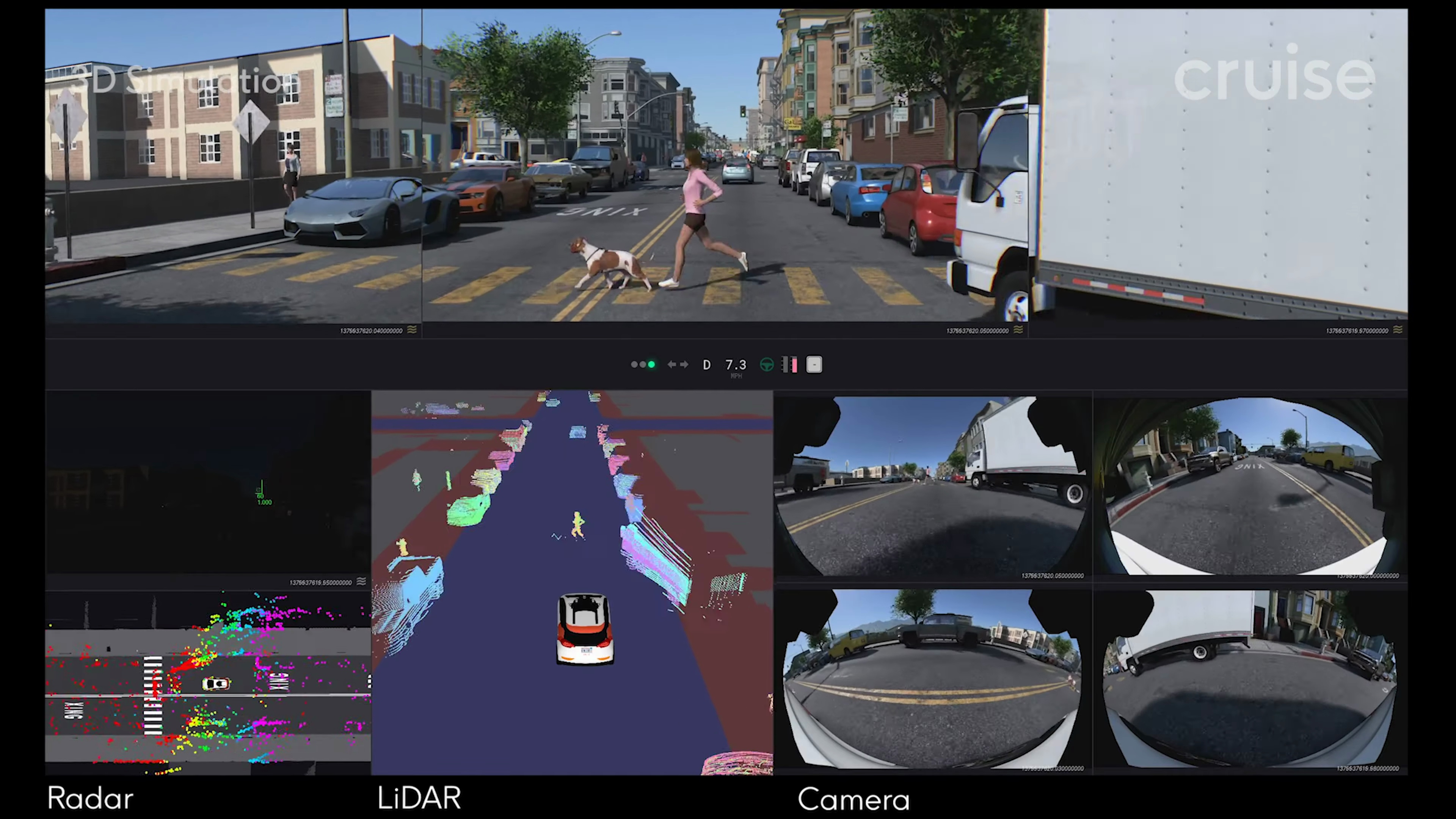
Example of Cruise’s synthetic simulation showing the same scene rendered into synthetic camera, lidar, and radar data. Source: Cruise.
For example, a Cruise blog post mentions some elements of their synthetic simulation roadmap (emphasis mine):
With limited time and resources, we have to make choices. For example, we ask how accurately we should model tires, and whether or not it is more important than other factors we have in our queue, like modeling LiDAR reflections off of car windshields and rearview mirrors or correctly modeling radar multipath returns.
Even if rendering reflections and translucent surfaces is already well understood in computer graphics, Cruise may still need to make sure their renderer generates realistic reflections that resemble their lidar. This challenge gives a sense of the attention to detail required. It’s only one of many that needs to be solved when building a synthetic sensor simulator.
So far, we have only covered the high development costs. Synthetic sensor simulation also incurs high variable costs every time simulation is run.
Round-trip conversions to pixels and back
By its nature, synthetic sensor simulation performs a round-trip conversion to and from synthetic imagery to test the perception system. The game engine first renders its scene description to synthetic imagery for each sensor on the simulated vehicle, burning many precious GPU-hours in the process, only to have the perception system perform the inverse operation when it detects the objects in the scene to produce the autonomous vehicle’s internal scene representation.5 Every time you launch a synthetic sensor simulation, NVIDIA, Intel, and/or AWS are laughing all the way to the bank.
Despite the expense of testing the perception system with synthetic simulation, it is also arguably less effective than testing with real-world imagery paired with ground truth labels. With real imagery, there can be no question about its realism. Synthetic imagery never looks quite right.
These practical limitations mean that synthetic sensor simulation ends up as the least used simulator type in AV companies. Usually, it’s also the last type of simulator to be built at a new company. Developers don’t need synthetic imagery most of the time, especially when they have at their disposal a fleet of vehicles that can record the real thing.
On the other hand, we cannot easily test risky driving behavior in the real world. For example, it is better to synthesize a bunch of red light runners than try to find them in the real world. This means we are primarily using synthetic simulation to test the behavior system.
Skipping the sensor data
In synthetic agent simulation, the simulator uses a high-level scene description to generate synthetic outputs from the perception/sensing system. In software development terms, it’s like replacing the perception system with a mock to focus on testing downstream components.
This type of simulation requires fewer computational resources to run because the scene description doesn’t need to make a round-trip conversion to sensor data.

Modified architecture diagram for running synthetic simulation with generated agents.
With image quality out of the picture, the value of synthetic simulation rests solely on the quality of the scenarios it can create. We can split this into two main challenges:
- designing agents with realistic behaviors
- generating the scene descriptions containing various agents, street layouts, and environmental conditions
Making smart agents
You could start developing the control policy for a smart agent similar to NPC design in early video games.
- A basic smart agent could simply follow a line or a path without reacting to anyone else, which could be used to test the autonomous vehicle’s reaction to a right of way violation.
- A fancier smart agent could follow a path while also maintaining a safe following distance from the vehicle in front. This type of agent could be placed behind our simulated vehicle, resolving the rear-ending problem mentioned above.
Like an audience of demanding gamers, the users of our simulator quickly expect increasingly complex and intelligent behaviors from the smart agents. An ideal smart agent system would capture the full spectrum of every action that other road users could possibly take. This system would also generate realistic behaviors, including realistic-looking trajectories and reaction times, so that we can trust the outcomes of simulations involving smart agents. Finally, our smart agents need to be controllable: they can be given destinations or intents, enabling developers to design simulations that test specific scenarios.
Two Cruise simulations in which smart agents (orange boxes) interact with the autonomous vehicle. In the second simulation, two parked cars have been inserted into the bottom of the visualization. Notice how the smart agents and the autonomous vehicle drive differently in the two simulations as they interact with each other and the additional parked cars. Source: Cruise.
Developing a great smart agent policy ends up falling in the same difficulty ballpark as developing a great autonomous driving policy. The two systems may even share technical foundations. For example, they may have a shared component that is trained to predict the behaviors of other road users, which can be used for both planning our vehicle’s actions and for generating realistic agents in simulation.
Generating scene descriptions
Even with the ability to generate realistic synthetic imagery and realistic smart agent behaviors, our synthetic simulation is not complete. We still need a broad and diverse dataset of scene descriptions that can thoroughly test our vehicle.
These scene descriptions usually come from a mix of sources:
- Automatic conversion from onroad scenarios: We can write a program that takes a logged real-world drive, guesses the intent of other road users, and stores those intents as a synthetic simulation scenario.
- Manual design: Analogous to a level editor in a video game. A human either builds the whole scenario from scratch or makes manual edits to an automatic conversion. For example, a human can design a scenario based on a police report of a human-on-human-driver collision to simulate what the vehicle might have done in that scenario.
- Generative AI: Recent work from Zoox uses diffusion models trained on a large dataset of onroad scenarios.
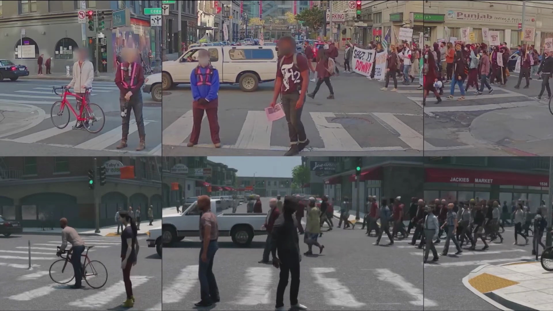
Example of a real-world log (top) converted to a synthetic simulation scenario, then rendered into synthetic camera images (bottom). Notice how some elements, such as the protest signs, are not carried over, perhaps because they are not supported by the perception system or the scene converter. Source: Cruise.
Scenarios can also be fuzzed, where the simulator adds random noise to the scene parameters, such as the speed limit of the road or the goals of simulated agents. This can upsample a small number of converted or manually designed scenes to a larger set that can be used to check for robustness and prevent overfitting.
Fuzzing can also help developers understand the space of possible outcomes, as shown in the example below, which fuzzes the reaction time of a synthetic tailgater:
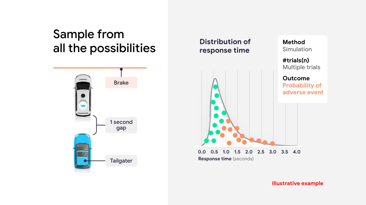
An example of fuzzing tailgater reaction time. Source: Waymo.
The distribution on the right shows a dot for each variant of the scenario, colored green or red depending on whether a simulated collision occurred. In this experiment, the collision becomes unavoidable once the simulated tailgater’s reaction time exceeds about 1 second.
Limitations of pure synthetic simulation
With these sources plus fuzzing, we’ve ensured the quantity of scenarios in our library, but we still don’t have any guarantees on the quality.
Perhaps the scenarios we (and maybe our generative AI tools) invent are too hard or too easy compared to the distribution of onroad driving our vehicle encounters.
- If our vehicle drives poorly in a synthetic scenario, does the autonomous driving system need improvement? Or is the scenario unrealistically hard, perhaps because the behavior of its smart agents is too unreasonable?
- If our vehicle passes with flying colors, is it doing a good job? Or is the scenario library missing some challenging scenarios simply because we did not imagine that they could happen?
This is a fundamental problem of pure synthetic simulation. Once we start modifying and fuzzing our simulated scenarios, there isn’t a straightforward way to know whether they remain representative of the real world. And we still need to collect a large quantity of real-world mileage to ensure that we have not missed any rare scenarios.
Hybrid simulation
We can combine our two types of simulator into a hybrid simulator that takes advantages of the strengths of each, providing an environment that is both realistic and interactive without breaking the bank.
- From replay simulation, use log replay to ensure every simulated scenario is rooted in a real-world scenario and has perfectly realistic sensor data.
- From synthetic simulation, make the simulation interactive by selectively replacing other road users with smart agents if they could interact with our vehicle.6

Modified architecture diagram merging parts of replay and synthetic simulation.
Hybrid simulation usually serves as the default type of simulation that works well for most use cases. One convenient interpretation is that hybrid simulation is a worry-free replacement for replay simulation: anytime the developer would have used replay, they can absentmindedly switch to hybrid simulation to take care of the most common simulation artifacts while retaining most of the benefits of replay simulation.
Conclusion
We’ve seen that there are many types of simulation used in autonomous driving. They exist on a spectrum from purely replaying onroad scenarios to fully synthesized environments. The ideal simulation platform allows developers to pick an operating point on that spectrum that fits their use case. Hybrid simulation based on a large volume of real-world miles satisfies most testing needs at a reasonable cost, while fully synthetic modes serve niche use cases that can justify the higher development and operating costs.
-
Cruise has written several deep dives about the usage and scaling of their simulation platform. However, neither Cruise nor Waymo provide many details on the construction of their simulator. ↩
-
I’ve even heard arguments that it’s only good for making videos. ↩
-
There exist architectures that are more end-to-end. However, to the best of my knowledge, those systems do not have driverless deployments with nontrivial mileage, making simulation testing less relevant. ↩
-
Another interactivity problem arises from the replay simulator’s inability to simulate different points of view as the simulated vehicle moves. A large pose divergence often causes the simulated vehicle to drive into an area not observed by the vehicle that produced the onroad log. For example, a simulated vehicle could decide to drive around a corner much earlier. But it wouldn’t be able to see anything until the log data also rounds the corner. No matter where the simulated vehicle drives, it will always be limited to what the logged vehicle saw. ↩
-
“Computer vision is inverse computer graphics.” ↩
-
As a nice bonus, because the irrelevant road users are replayed exactly as they drove in real life, this may reduce the compute cost of simulation. ↩